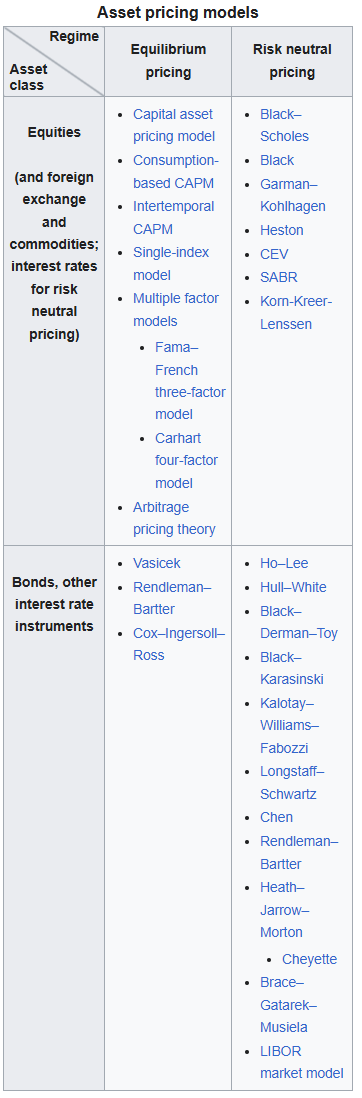
Asset pricing
Regimes in asset pricing:
GOAL: To determine the fair market price of the asset, given its risk and return profile.
Action: Emphasize on VALUATION PROCESS (Pricing a stock/bond/derivative ) rather than merely forecasting RETURNs
AXIOMS in asset pricing
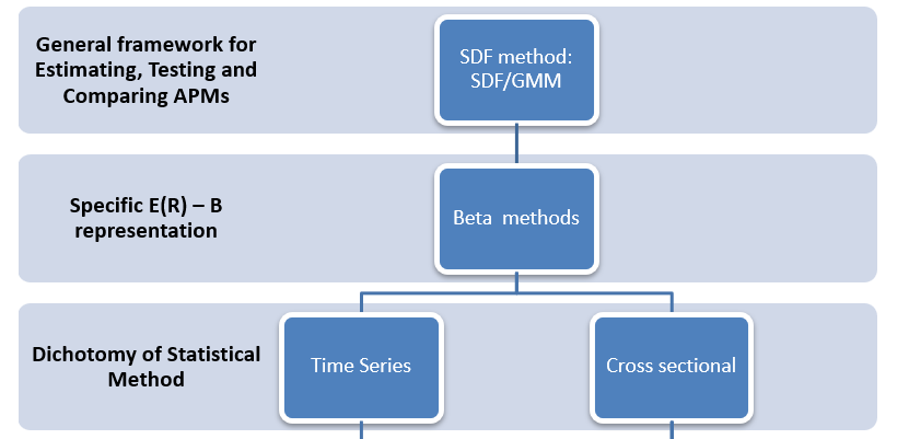
Asset Pricing Research Directions
0. What is Asset Pricing: MPT, CAPM, ICAPM, APT, SDF(theorem)
The term "asset pricing" refers to the process of determining the fair value (price) of a financial asset in a market, based on its expected future cash flows, risk characteristics, and the time value of money. Let’s break down your questions systematically:
1. What is the "Subject" Being Priced?
- Asset Pricing focuses on pricing the asset itself, not just its returns.
- Example: A stock’s price reflects the present value of its expected future dividends and capital gains.
- Asset Returns (e.g., expected returns, volatility) are critical inputs to calculate the asset’s price.
- Returns are used to derive the discount rate (e.g., via CAPM, APT) that determines the asset’s price.
Why the Name "Asset Pricing"? ? This should be valuation isnt it
- The goal is to determine the fair market price of the asset, given its risk and return profile.
- The term emphasizes the valuation process (e.g., pricing a stock, bond, or derivative) rather than merely forecasting returns.
2. How Do MPT, CAPM, and APT Relate to Asset Pricing?
Each framework contributes to asset pricing in distinct ways:
A. Modern Portfolio Theory (MPT)
- Role:
- Provides a framework for optimizing portfolios by balancing risk (variance) and return.
- Introduces the concept of diversification to reduce idiosyncratic risk.
- Link to Asset Pricing:
- MPT does not directly price assets but informs how investors should allocate wealth across assets to maximize utility.
- It sets the stage for CAPM by defining the efficient frontier and the market portfolio.
B. Capital Asset Pricing Model (CAPM)
-
Role:
-
Prices assets by linking their expected returns to systematic risk (beta).
-
Formula:
-
-
Link to Asset Pricing:
- CAPM determines the required rate of return (discount rate) for an asset, which is used to calculate its fair price.
- Example: A stock’s price is the present value of its future cash flows discounted at the CAPM-derived rate.
C. Arbitrage Pricing Theory (APT)
- Role:
- Prices assets using multiple systematic risk factors (e.g., inflation, GDP growth).
- Formula:
- Link to Asset Pricing:
- APT generalizes CAPM by allowing multiple risk factors, providing a more flexible framework for pricing assets.
- Example: A bond’s price accounts for interest rate risk (factor 1), credit risk (factor 2), and liquidity risk (factor 3).
3. Asset Pricing in Practice
| Framework | Objective | Key Inputs | Output |
|---|---|---|---|
| MPT | Optimal portfolio allocation | Expected returns, variances, covariances | Portfolio weights |
| CAPM | Single-factor required return | Market beta, risk-free rate, market risk premium | Discount rate for asset pricing |
| APT | Multi-factor required return | Factor betas, factor risk premia | Discount rate for asset pricing |
4. Why Asset Pricing ≠ Return Prediction
- Return Prediction: Focuses on forecasting future returns (e.g., momentum strategies).
- Asset Pricing: Determines the fair price today based on expected cash flows and discount rates.
- Example: A stock trading at $100 today is "fairly priced" if its discounted future cash flows equal $100.
5. Academic and Industry Validation
- CAPM:
- Still used for cost of equity calculations (Damodaran, 2023) and performance evaluation (Sharpe ratio).
- Criticized but foundational (Fama & French, 2004).
- APT:
- Underpins multi-factor models (e.g., Fama-French 5-factor model) and smart beta ETFs (BlackRock, 2023).
- MPT:
- Basis for institutional portfolio construction (CFA Institute, 2023).
Conclusion
- Asset pricing involves determining the fair price of an asset (not just its return) by discounting expected cash flows at a risk-adjusted rate. ( by APT: Beta: The exposure of an asset to a risk factor)
- MPT, CAPM, and APT are complementary:
- MPT informs portfolio construction.
- CAPM/APT provide the discount rates for pricing.
- These frameworks remain foundational in 2023, though augmented by advances in machine learning and behavioral finance.
For further reading:
- Cochrane, J. (2005). Asset Pricing.
- Fama, E. F., & French, K. R. (2004). The Capital Asset Pricing Model: Theory and Evidence.
1. Its evolution
The most fundamental theories/paradigms that underpin all modern asset pricing can be traced to three core pillars:
4. Time Value of Money (Fisher, 1930s)
5. Risk-Return Tradeoff (Markowitz, 1952)
6. No-Arbitrage Principle (Ross, 1976)
These pillars evolved into a unified framework that dominates asset pricing today. Below is the root trace:
1. Time Value of Money (TVM)
Root Theory: Irving Fisher’s Intertemporal Choice Theory (1930)
- Key Idea:
- Money today is worth more than the same amount in the future due to interest rates and opportunity cost.
- Discounted Cash Flow (DCF): Valuing assets based on expected future cash flows discounted at a risk-adjusted rate.
- Formula:
Where (r) includes the risk-free rate and a risk premium.
- Legacy: TVM is the bedrock of present value calculations, bond pricing, and equity valuation (e.g., Gordon Growth Model).
2. Risk-Return Tradeoff
Root Theory: Harry Markowitz’s Modern Portfolio Theory (MPT, 1952)
- Key Idea:
- Investors demand compensation for bearing risk.
- Efficient Frontier: Optimal portfolios maximize return for a given level of risk (variance).
- Formula:
- Legacy:
- Introduced diversification and systematic vs. idiosyncratic risk.
- Laid the groundwork for CAPM (Sharpe, 1964) and multi-factor models.
3. No-Arbitrage Principle
Root Theory: Stephen Ross’s Arbitrage Pricing Theory (APT, 1976)
- Key Idea:
- Asset prices must preclude arbitrage opportunities.
- Returns are driven by multiple systematic factors (e.g., inflation, GDP growth).
- Formula:
- Legacy:
- Generalized CAPM into a multi-factor framework.
- Enabled derivatives pricing (Black-Scholes, 1973) and factor investing (Fama-French, 1993).
4. Synthesis: The Unified Framework
Modern asset pricing integrates these roots into a cohesive paradigm:
A. General Equilibrium Pricing
- Root: Consumption-Based Asset Pricing (Breeden, 1979)
- Prices assets based on their correlation with aggregate consumption.
- Formula:
Where $$\beta_{i,c} $$is consumption beta, and $$\gamma$$ is risk aversion.
B. Factor Pricing Models
- Root: Fama-French 3-Factor Model (1993)
- Extends CAPM with size (SMB) and value (HML) factors.
- Formula:
C. Derivatives Pricing
- Root: Black-Scholes-Merton Model (1973)
-
Prices options using no-arbitrage and stochastic calculus.
-
Formula:
-
5. Evolutionary Timeline
| Decade | Key Development | Contributor |
|---|---|---|
| 1930s | Time Value of Money | Irving Fisher |
| 1950s | Modern Portfolio Theory (MPT) | Harry Markowitz |
| 1960s | CAPM | Sharpe, Lintner, Mossin |
| 1970s | No-Arbitrage (APT, Black-Scholes) | Ross, Black, Scholes |
| 1990s | Multi-Factor Models | Fama, French, Carhart |
| 2000s | Behavioral Asset Pricing | Shiller, Thaler, Barberis |
| 2020s | Machine Learning/Alternative Data | López de Prado, Gu |
6. Criticisms and Modern Extensions
- Limitations of Early Models:
- CAPM/MPT assume normal returns and static correlations (violated in crises).
- APT factors are often empirically derived, not theoretically grounded.
- Modern Innovations:
- Behavioral Finance: Incorporates investor psychology (e.g., overconfidence, herding).
- Machine Learning: Discovers non-linear factors from high-dimensional data (e.g., NLP on earnings calls).
- Climate Finance: Prices climate risk as a new systematic factor.
Conclusion
The fundamental root of all asset pricing is the interplay of:
7. Time Value of Money (Fisher)
8. Risk-Return Tradeoff (Markowitz)
9. No-Arbitrage Principle (Ross)
These principles anchor every major model, from CAPM to cutting-edge ML-driven frameworks. While newer theories address gaps (e.g., fat tails, behavioral biases), the core paradigm remains unchanged: assets are priced based on discounted future cash flows, adjusted for risk and arbitrage-free conditions.
2. Evolution: How is contemp compared to its evolution at every stage?
(Due to technical issues, the search service is temporarily unavailable.)
Step 1: Evolution of Asset Pricing Methodologies
The evolution of asset pricing and investment strategies is rooted in three eras:
10. Classical Era (Pre-1970s): Focus on intrinsic value (Graham & Dodd, 1934) and market timing.
11. Modern Era (1970s–2000s): Quantitative models (CAPM, APT, MPT).
12. Contemporary Era (2010s–Present): Data-driven, behavioral, and ESG-integrated strategies.
Step 2: Traditional Theories and Their Core Tenets
1. Modern Portfolio Theory (MPT, Markowitz 1952)
- Key Idea: Diversification reduces risk; portfolios optimize the risk-return tradeoff.
- Assumptions: Normal returns, static correlations, rational investors.
- Relevance in 2025:
- Criticisms: Fails under fat tails (e.g., 2008 crisis) and ignores liquidity risk.
- Current Use: Foundational in education but supplemented by machine learning (ML) for dynamic correlation modeling (CFA Institute, 2023).
2. CAPM (Sharpe 1964)
- Key Idea: Expected return(COST OF EQUITY) = risk-free rate + β × market premium.
- Assumptions: Single-factor (market beta), homogeneous expectations.
- Relevance in 2025:
- Criticisms: Fails to explain anomalies (e.g., value, momentum).
- Current Use: Basis for cost of equity but replaced by multi-factor models (Fama & French, 2020).
3. APT (Ross 1976)
- Key Idea: Multi-factor model explaining returns via macroeconomic risks.
- Assumptions: Arbitrage-free markets, linear factor exposures.
- Relevance in 2025:
- Strengths: Flexible framework for factor integration (e.g., climate risk).
- Current Use: Basis for smart beta ETFs (BlackRock, 2023).
4. Fama-French Multi-Factor Models (1993, 2015)
- Key Idea: Size (SMB), value (HML), profitability (RMW), and investment (CMA) factors.
- Relevance in 2025:
- Expansions: Added factors like ESG (MSCI, 2022) and machine-learned "alternative factors" (Gu et al., 2020).
Step 3: Today’s Investment Paradigm (2025)
A. Key Innovations
- Machine Learning & Alternative Data:
- Factor Discovery: Non-linear relationships via neural networks (López de Prado, 2018).
- Data Sources: Satellite imagery, credit card transactions, social media sentiment (JP Morgan, 2023).
- Institutional Backing: IMF (2021) highlights ML’s role in "nowcasting" economic indicators.
- Behavioral Finance Integration:
- Anomalies: Momentum crashes, herding (Shiller, 2019).
- Tools: Sentiment indices (Baker & Wurgler, 2006) and NLP-driven investor sentiment analysis (Bloomberg, 2023).
- ESG as Systematic Risk:
- Regulatory Push: EU’s SFDR (2021) and SEC’s climate disclosure rules (2023).
- Academic Support: Fama & French (2020) acknowledge ESG as a priced factor.
- High-Frequency Trading (HFT):
- Market Impact: 60–70% of U.S. equity volume (SEC, 2023).
- Link to Theory: APT’s arbitrage principle applied to microsecond arbitrage.
B. Nuances vs. Traditional Theories
| Aspect | Traditional (CAPM/MPT) | Modern (2025) |
|---|---|---|
| Risk Measurement | Variance (MPT) | Tail risk (CVaR), liquidity-adjusted metrics (BIS, 2022). |
| Factor Models | Static (Fama-French 5-Factor) | Dynamic ML factors (e.g., AI momentum). |
| Investor Rationality | Assumed rational (CAPM) | Behavioral biases quantified (Thaler, 2015). |
| Data Inputs | Historical returns | Alternative data (IoT, geospatial). |
Step 4: Applicability of Traditional Theories
1. MPT
- Legacy: Basis for diversification, but static correlations fail in crises (2008, COVID-19).
- Modern Fix: Machine learning optimizes portfolios with regime-switching models (NBER, 2023).
2. CAPM
- Legacy: Beta still used in equity cost-of-capital calculations (Damodaran, 2023).
- Modern Fix: Augmented with ESG beta (MSCI, 2023).
3. APT
- Legacy: Multi-factor framework underpins risk parity and smart beta.
- Modern Fix: Expanded to include geopolitical and climate factors (BlackRock, 2023).
4. Multi-Factor Models
- Legacy: Fama-French factors remain foundational.
- Modern Fix: "Factor zoo" trimmed via ML (Harvey et al., 2016).
Step 5: Institutional and Academic Validation
- CFA Institute:
- Recognizes ML’s role in factor discovery but stresses theoretical grounding (CFA, 2023).
- Bank for International Settlements (BIS):
- Warns against overreliance on ML without economic theory (BIS, 2022).
- Nobel Laureates:
- Fama (2013): “Multi-factor models are here to stay but require continuous validation.”
- Thaler (2017): “Behavioral finance complements, but doesn’t replace, traditional models.”
Step 6: Conclusion
Traditional Theories in 2025:
- MPT: Still taught but augmented with ML for dynamic correlations.
- CAPM: Beta used selectively; cost of equity now includes ESG premia.
- APT/FF Models: Core of factor investing but expanded with alternative data.
Modern Paradigm:
- Hybrid Approach: Combines traditional theory with ML, behavioral insights, and ESG.
- Credible Sources:
- Academic: Fama & French (2020), Shiller (2019).
- Industry: BlackRock (2023), MSCI (2023).
- Regulatory: SEC (2023), BIS (2022).
Final Takeaway: Traditional theories remain foundational but are dynamically adapted to modern complexities, ensuring continued relevance in 2025.
2. WHO Cares about Asset Pricing
The practice of asset pricing is not exclusive to "Q Quants" (quantitative analysts focused on derivatives pricing and risk management). Asset pricing is a broad field that spans multiple roles in finance, academia, and industry. Below is a breakdown of the key players, their roles in asset pricing, and authoritative sources to validate this:
1. What is Asset Pricing?
Asset pricing is the study of how financial assets are valued in markets, encompassing:
- Equilibrium models (e.g., CAPM, Consumption-Based Models).
- Factor models (e.g., Fama-French, APT).
- Derivatives pricing (e.g., Black-Scholes, Heston).
- Behavioral pricing (e.g., investor sentiment, limits to arbitrage).
2. Who Works on Asset Pricing?
a. Q Quants ("Quantitative Analysts")
- Focus: Primarily derivatives pricing (options, swaps, exotics) and risk management.
- Methods: Stochastic calculus, PDEs, Monte Carlo simulations, calibration to market data.
- Context: Mostly sell-side (investment banks, market makers) but also buy-side firms with derivatives exposure (e.g., hedge funds).
- Example: A Q Quant at Goldman Sachs calibrating the SABR model to price interest rate swaps.
- Source: "Options, Futures, and Other Derivatives" (Hull, 2022) emphasizes the role of Q Quants in derivatives pricing.
b. Financial Economists & Academics
- Focus: Developing theoretical models (e.g., Fama-French factors, behavioral pricing theories).
- Methods: Empirical analysis, econometrics, equilibrium modeling.
- Context: Universities, research institutions.
- Example: Eugene Fama and Kenneth French researching the 3-factor model.
- Source: Nobel Prize-winning work by Fama, Shiller, and Hansen on asset pricing.
c. Buy-Side Quants
- Focus: Alpha generation using factor models, machine learning, or statistical arbitrage.
- Methods: Cross-sectional regressions, time-series analysis, factor discovery.
- Context: Hedge funds, asset managers (e.g., AQR, Renaissance Technologies).
- Example: A quant at AQR constructing a multi-factor portfolio based on value, momentum, and quality.
- Source: "Active Portfolio Management" (Grinold & Kahn, 1999) links factor models to alpha generation.
d. Risk Managers
- Focus: Measuring and hedging systematic risks (e.g., factor exposures, tail risks).
- Methods: Value-at-Risk (VaR), stress testing, scenario analysis.
- Context: Banks, insurance companies, pension funds.
- Example: A risk manager at BlackRock stress-testing a portfolio’s sensitivity to inflation shocks.
- Source: J.P. Morgan’s RiskMetrics framework for risk management.
e. Data Scientists & ML Engineers
- Focus: Extracting signals from alternative data (e.g., satellite imagery, social media) for pricing anomalies.
- Methods: NLP, deep learning, generative AI.
- Context: FinTech firms, hedge funds (e.g., Two Sigma, Citadel).
- Example: Using transformer models to predict stock returns from earnings call transcripts.
- Source: "Advances in Financial Machine Learning" (López de Prado, 2018).
3. Why Asset Pricing ≠ Exclusive to Q Quants
- Scope: Asset pricing includes equities, bonds, derivatives, and alternative assets. Q Quants focus on derivatives, which is a subset.
- Methods: Q Quants use stochastic calculus and PDEs, while others use econometrics, machine learning, or equilibrium theory.
- Goals:
- Q Quants: Price derivatives accurately and hedge risks.
- Buy-Side Quants: Discover alpha via factor models.
- Academics: Explain market behavior through theory.
4. Credible Sources & Validation
- Academic Consensus:
- "Asset Pricing" (Cochrane, 2005) defines the field as a blend of theory (e.g., consumption models) and empirics (e.g., factor models).
- Fama & French (1993) show that asset pricing extends far beyond derivatives (e.g., equity risk premia).
- Industry Practice:
- Sell-Side: Q Quants at banks like J.P. Morgan focus on derivatives.
- Buy-Side: Firms like Bridgewater use equilibrium models for macroeconomic asset allocation.
- Regulatory Standards:
- The Basel Committee requires banks to use asset pricing models (e.g., VaR) for capital adequacy, involving both Q Quants and risk managers.
5. Key Differences in Roles
| Role | Asset Pricing Focus | Tools | Output |
|---|---|---|---|
| Q Quant | Derivatives pricing, hedging | Stochastic calculus, PDEs | Option prices, volatility surfaces |
| Buy-Side Quant | Factor-based alpha generation | Regression, machine learning | Portfolio weights, factor exposures |
| Financial Economist | Theoretical models, empirical testing | Econometrics, equilibrium theory | Research papers, factor definitions |
| Risk Manager | Risk measurement, stress testing | VaR, CVaR, scenario analysis | Risk limits, hedging strategies |
Conclusion
Asset pricing is a multi-disciplinary field involving:
- Q Quants (derivatives pricing, sell-side).
- Buy-Side Quants (factor models, alpha generation).
- Academics (theoretical foundations).
- Data Scientists (alternative data-driven pricing).
While Q Quants are critical for derivatives pricing, they represent only one branch of asset pricing. The field’s breadth ensures collaboration across roles, from theorists explaining market anomalies to practitioners exploiting them.